visualize DE genes FRCs
Load packages
## load packages
suppressPackageStartupMessages({
  library(dplyr)
  library(reshape2)
  library(ggplot2)
  library(cowplot)
  library(purrr)
  library(Seurat)
  library(tidyverse)
  library(ggpubr)
  library(runSeurat3)
  library(here)
  library(ggsci)
  library(pheatmap)
  library(scater)
})
load seurat object
basedir <- here()

seurat <- readRDS(file= paste0(basedir,
                               "/data/AllPatWithoutCM_FRConly_intOrig_seurat.rds"))

## remove cluster with cycling cells
seurat <- subset(seurat, integrated_snn_res.0.25 == "8", invert=T)


DefaultAssay(object = seurat) <- "RNA"
seurat$intCluster <- as.character(seurat$integrated_snn_res.0.25)
Idents(seurat) <- seurat$intCluster


## set col palettes
colPal <- c(pal_uchicago()(6), "#6692a3", "#3b7f60")
names(colPal) <- c("0", "1", "2", "3", "4", "5", "6", "7")
colPat <- c(pal_nejm()(7),pal_futurama()(12))[1:length(unique(seurat$patient))]
names(colPat) <- unique(seurat$patient)
colCond <- c("#6692a3","#971c1c","#d17d67")
names(colCond) <- unique(seurat$cond)
colGrp <- pal_uchicago()(length(unique(seurat$grp)))
names(colGrp) <- unique(seurat$grp)
colOri <- pal_npg()(length(unique(seurat$origin)))
names(colOri) <- unique(seurat$origin)
colTon <- colCond

## all activated in one grp
seurat$cond2 <- seurat$cond
seurat$cond2[which(seurat$cond %in% c("chronic", "acute"))] <- "activated"

colCond2 <- c("#6692a3","#971c1c")
names(colCond2) <- c("resting", "activated")
visualize data
clustering
## visualize input data
DimPlot(seurat, reduction = "umap", cols=colPal)+
  theme_bw() +
  theme(axis.text = element_blank(), axis.ticks = element_blank(),
        panel.grid.minor = element_blank()) +
  xlab("UMAP1") +
  ylab("UMAP2")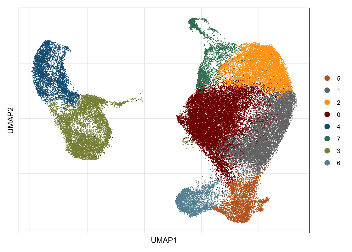
clustering split by cond2
DimPlot(seurat, reduction = "umap", cols=colPal, pt.size=0.5,
        split.by = "cond2")+
  theme_void()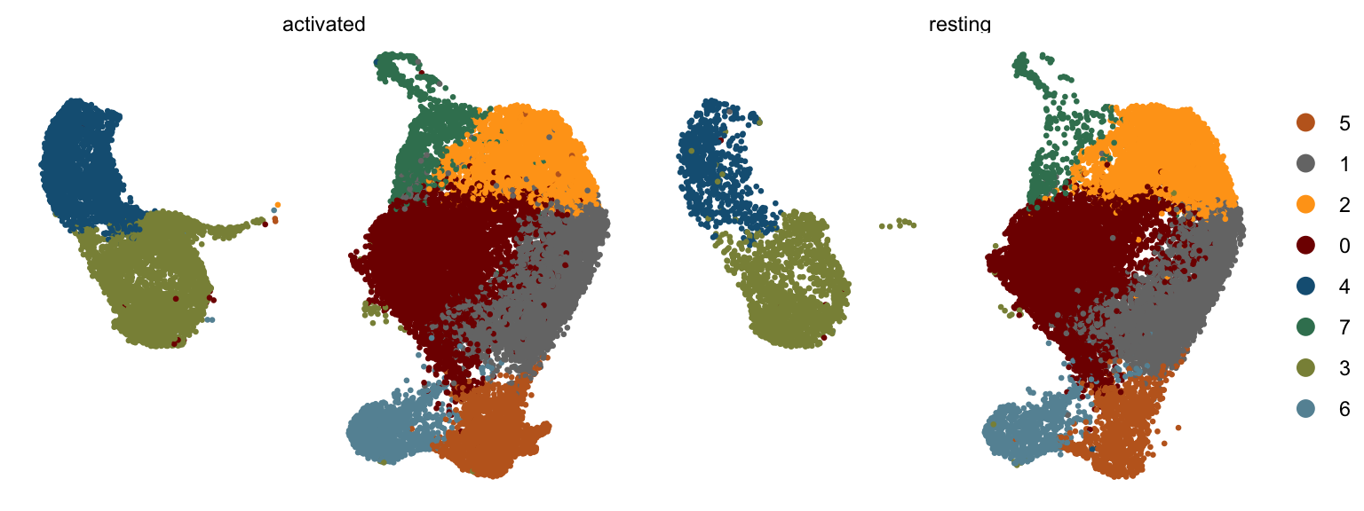
patient
## visualize input data
DimPlot(seurat, reduction = "umap", cols=colPat, group.by = "patient")+
  theme_bw() +
  theme(axis.text = element_blank(), axis.ticks = element_blank(),
        panel.grid.minor = element_blank()) +
  xlab("UMAP1") +
  ylab("UMAP2")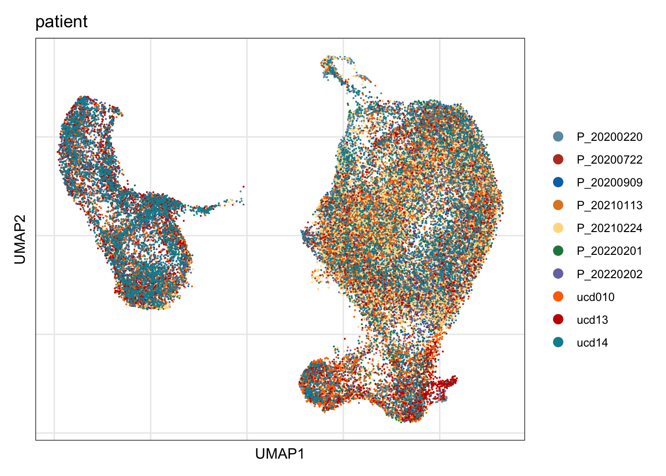
cond
## visualize input data
DimPlot(seurat, reduction = "umap", cols=colCond, group.by = "cond")+
  theme_bw() +
  theme(axis.text = element_blank(), axis.ticks = element_blank(),
        panel.grid.minor = element_blank()) +
  xlab("UMAP1") +
  ylab("UMAP2")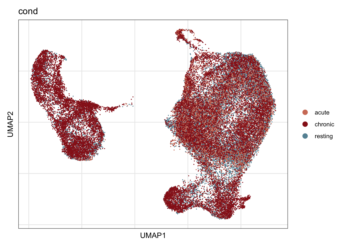
cond2
## visualize input data
DimPlot(seurat, reduction = "umap", cols=colCond2, group.by = "cond2",
        shuffle = T)+
  theme_bw() +
  theme(axis.text = element_blank(), axis.ticks = element_blank(),
        panel.grid.minor = element_blank()) +
  xlab("UMAP1") +
  ylab("UMAP2")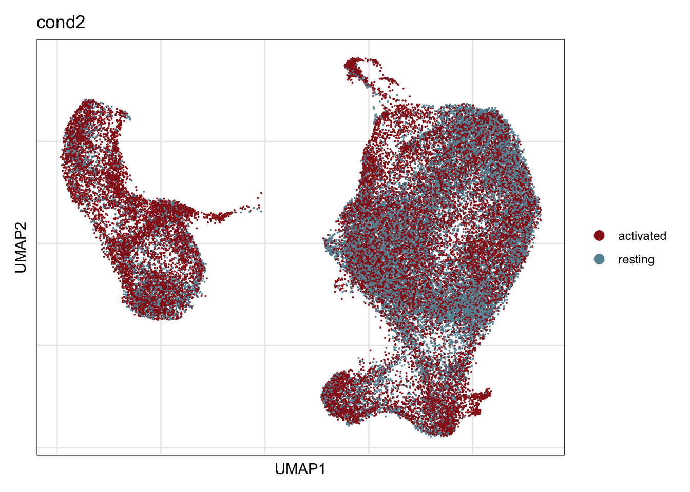
DimPlot(seurat, reduction = "umap", cols=colCond2, group.by = "cond2",
        pt.size=0.5, shuffle = T)+
  theme_void()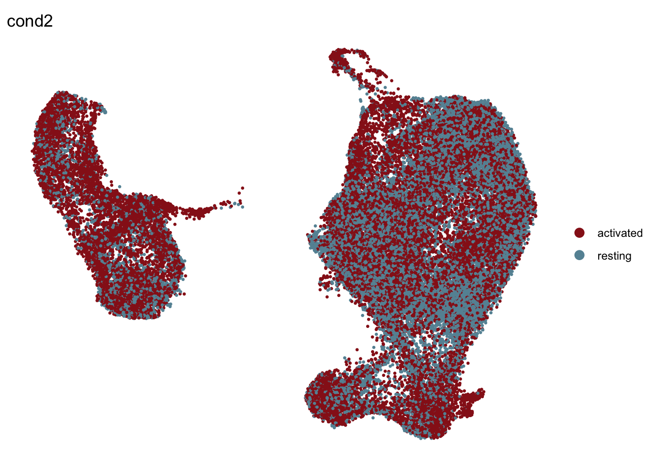
grp
## visualize input data
DimPlot(seurat, reduction = "umap", cols=colGrp, group.by = "grp")+
  theme_bw() +
  theme(axis.text = element_blank(), axis.ticks = element_blank(),
        panel.grid.minor = element_blank()) +
  xlab("UMAP1") +
  ylab("UMAP2")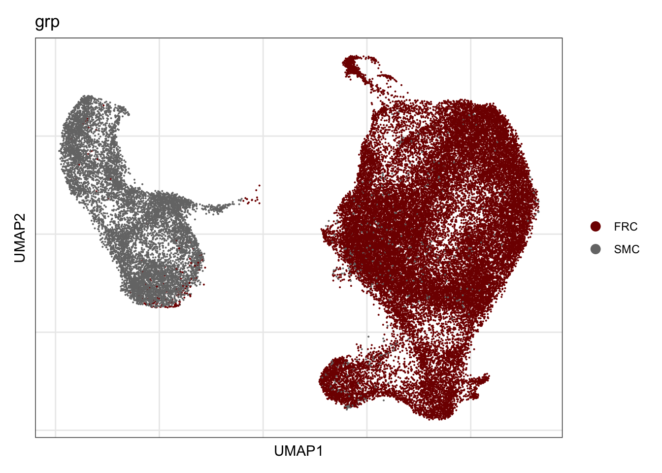
origin
## visualize input data
DimPlot(seurat, reduction = "umap", cols=colOri, group.by = "origin")+
  theme_bw() +
  theme(axis.text = element_blank(), axis.ticks = element_blank(),
        panel.grid.minor = element_blank()) +
  xlab("UMAP1") +
  ylab("UMAP2")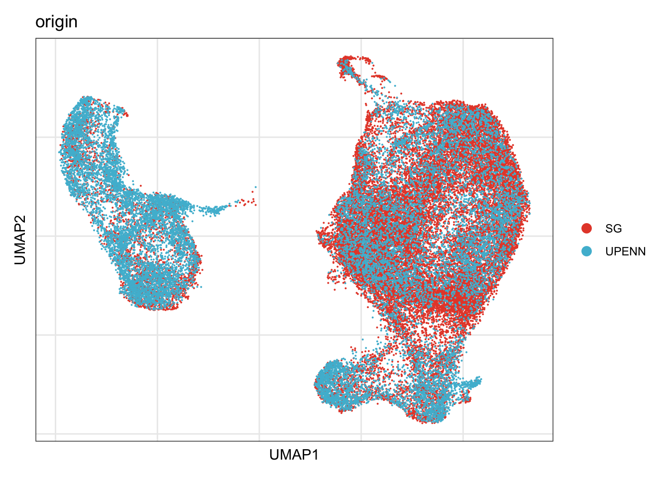
relative cluster abundances per cond2
clustCond <- data.frame(table(seurat$cond2, seurat$intCluster))
colnames(clustCond) <- c("cond", "intCluster", "cnt")
clustTot <- data.frame(table(seurat$intCluster))
colnames(clustTot) <- c("intCluster", "tot")
clustDat <- clustCond %>%  left_join(., clustTot, by = "intCluster") %>%
  mutate(relAb = cnt/tot * 100)

ggbarplot(clustDat, x="intCluster", y="relAb",
          fill="cond",
          colour= "cond",
          palette = colCond2,
          xlab = "cluster",
          ylab = "percentage")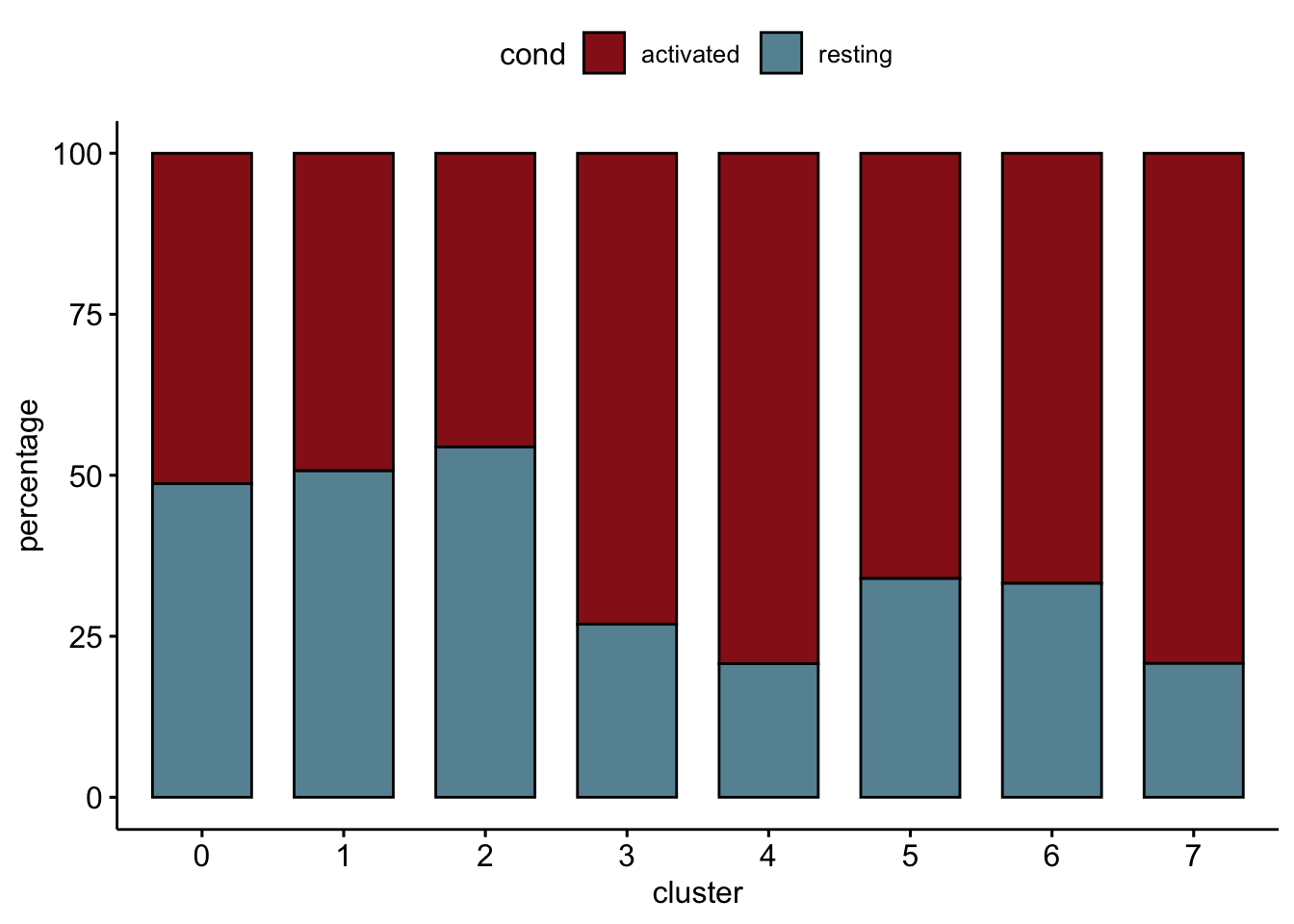
## relative abundance per cond
clustCond <- data.frame(table(seurat$cond2, seurat$intCluster))
colnames(clustCond) <- c("cond", "intCluster", "cnt")
condTot <- data.frame(table(seurat$cond2))
colnames(condTot) <- c("cond", "tot")
colPaldat <- data.frame(col=colPal) %>%
  rownames_to_column(var = "intCluster")
clustDat2 <- clustCond %>%  left_join(., condTot, by = "cond") %>%
  mutate(relAb = cnt/tot * 100) %>%
  left_join(., colPaldat, by = "intCluster")

knitr::kable(clustDat2)| cond | intCluster | cnt | tot | relAb | col |
|---|---|---|---|---|---|
| activated | 0 | 6373 | 25449 | 25.042241 | #800000FF |
| resting | 0 | 6049 | 18322 | 33.014955 | #800000FF |
| activated | 1 | 3969 | 25449 | 15.595898 | #767676FF |
| resting | 1 | 4080 | 18322 | 22.268311 | #767676FF |
| activated | 2 | 3164 | 25449 | 12.432709 | #FFA319FF |
| resting | 2 | 3773 | 18322 | 20.592730 | #FFA319FF |
| activated | 3 | 4244 | 25449 | 16.676490 | #8A9045FF |
| resting | 3 | 1560 | 18322 | 8.514354 | #8A9045FF |
| activated | 4 | 2767 | 25449 | 10.872726 | #155F83FF |
| resting | 4 | 724 | 18322 | 3.951534 | #155F83FF |
| activated | 5 | 1917 | 25449 | 7.532712 | #C16622FF |
| resting | 5 | 986 | 18322 | 5.381509 | #C16622FF |
| activated | 6 | 1528 | 25449 | 6.004165 | #6692a3 |
| resting | 6 | 760 | 18322 | 4.148019 | #6692a3 |
| activated | 7 | 1487 | 25449 | 5.843059 | #3b7f60 |
| resting | 7 | 390 | 18322 | 2.128589 | #3b7f60 |
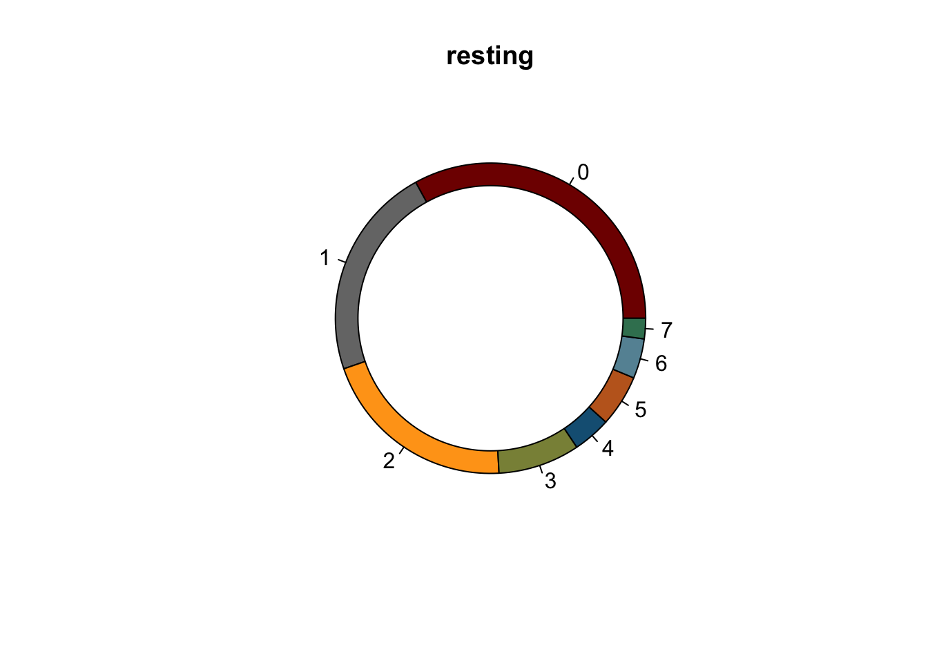
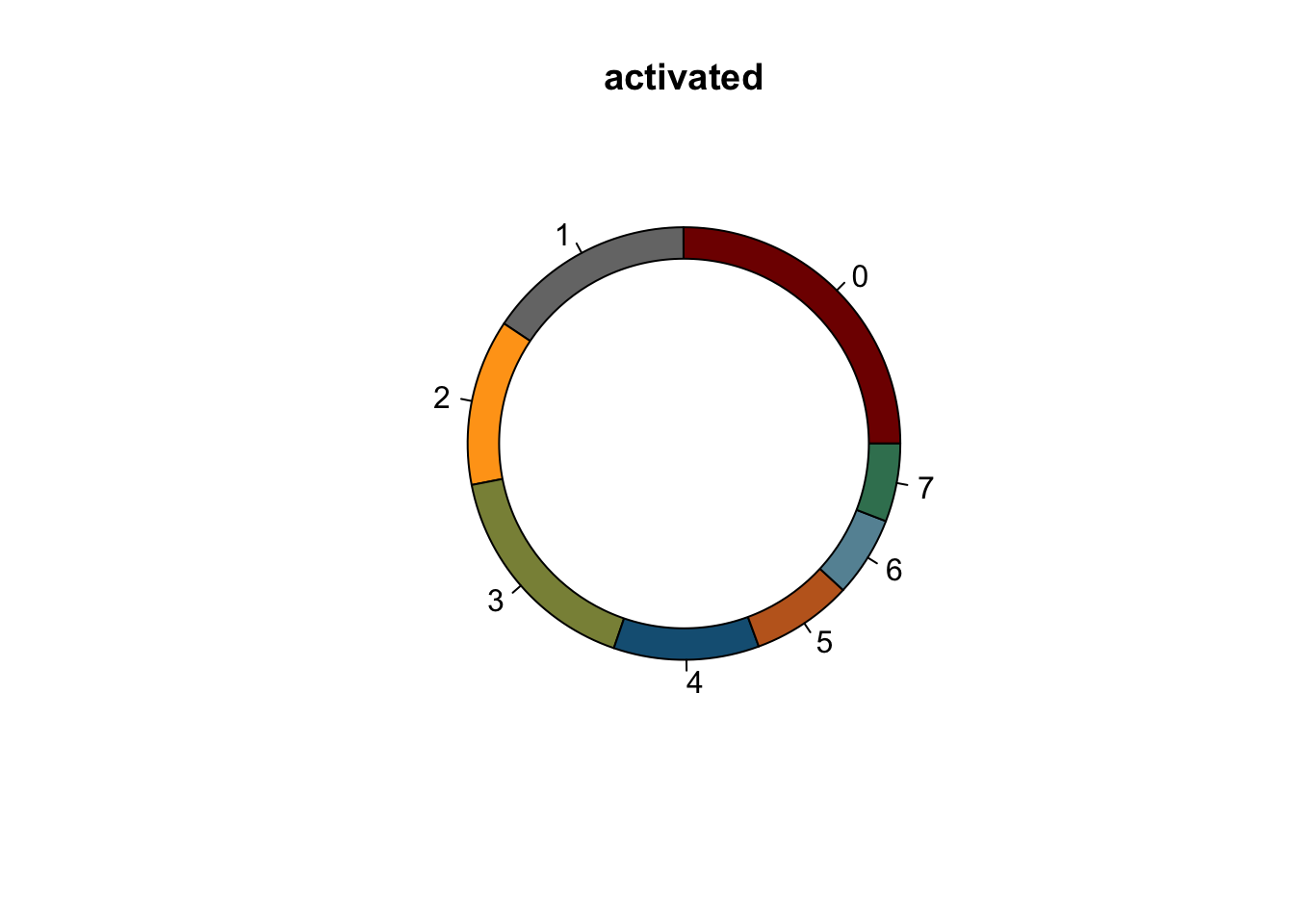
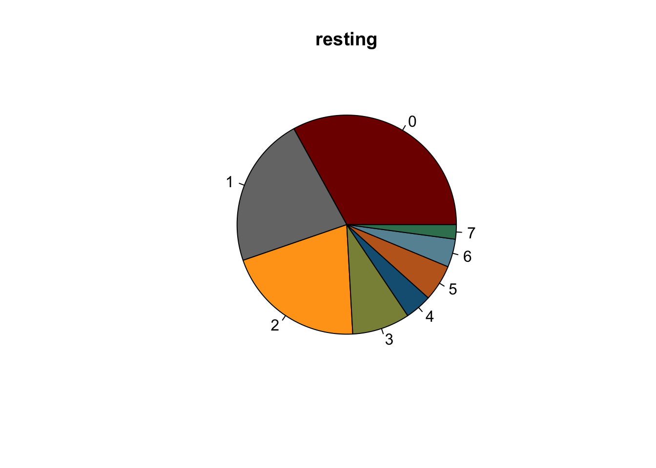
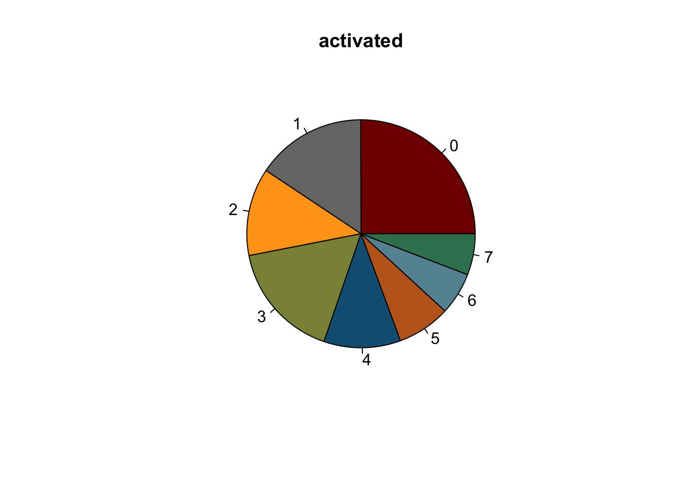
lapply(names(colCond2), function(co){
  clustDat2sel <- clustDat2 %>% filter(cond==co)
  pie(clustDat2sel$relAb,
      labels = clustDat2sel$intCluster,
      col = clustDat2sel$col,
      main = co)
  symbols(0, 0, circles = 1, add=TRUE, bg="white")
})
[[1]]
NULL

[[2]]
NULLlapply(names(colCond2), function(co){
clustDat2sel <- clustDat2 %>% filter(cond==co)
pie(clustDat2sel$relAb,
labels = clustDat2sel$intCluster,
col = clustDat2sel$col,
main = co)
})
[[1]]
NULL
[[2]]
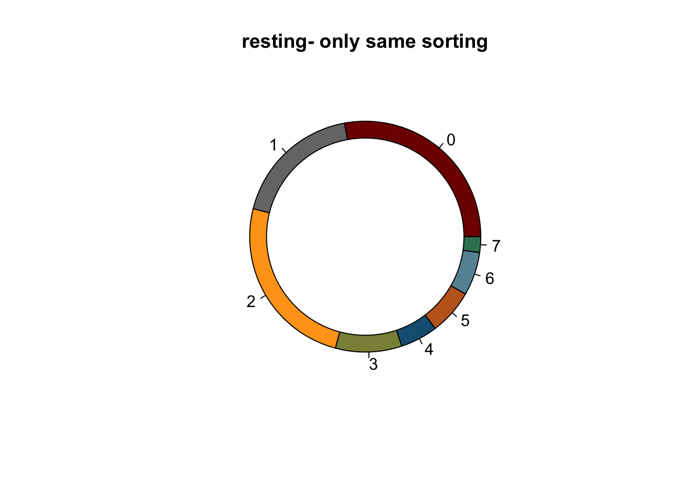
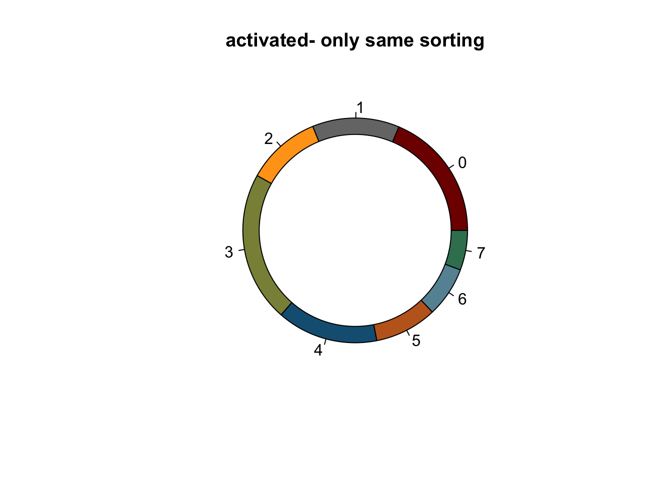
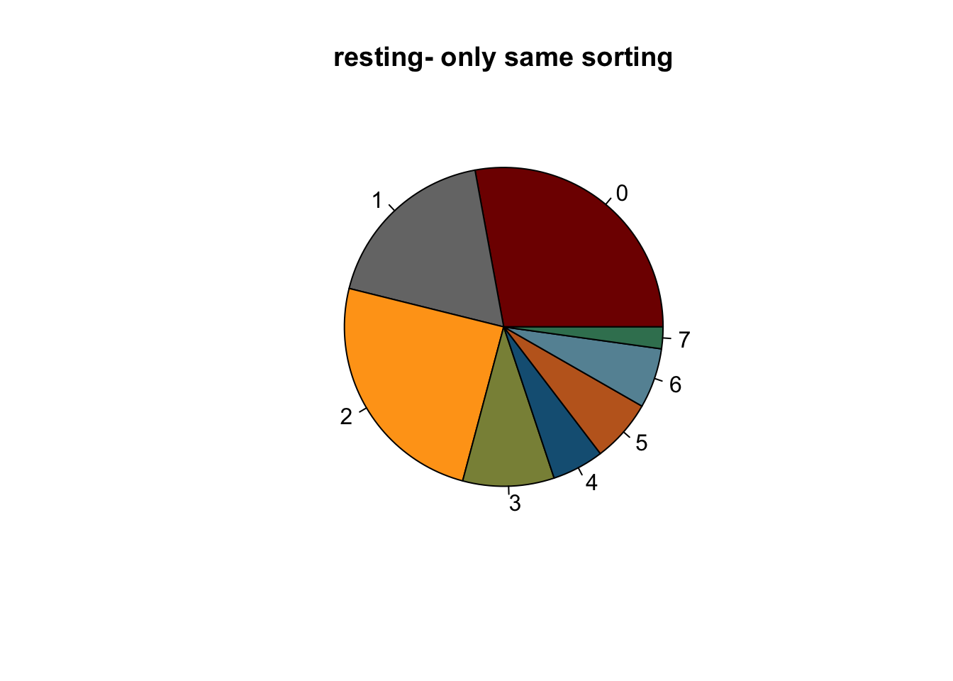
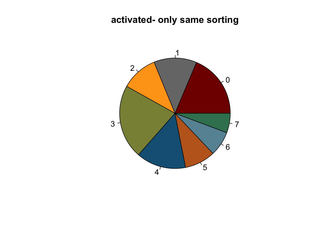
NULL### different sorting stratgies for the first samples..
seuratSub <- subset(seurat, patient %in% c("ucd010","ucd13","ucd14",
"P_20220201","P_20220202",
"P_20200220"))
clustCond <- data.frame(table(seuratSub$cond2, seuratSub$intCluster))
colnames(clustCond) <- c("cond", "intCluster", "cnt")
clustTot <- data.frame(table(seuratSub$intCluster))
colnames(clustTot) <- c("intCluster", "tot")
clustDat <- clustCond %>% left_join(., clustTot, by = "intCluster") %>%
mutate(relAb = cnt/tot * 100)
ggbarplot(clustDat, x="intCluster", y="relAb",
fill="cond",
colour= "cond",
palette = colCond2,
xlab = "cluster",
ylab = "percentage")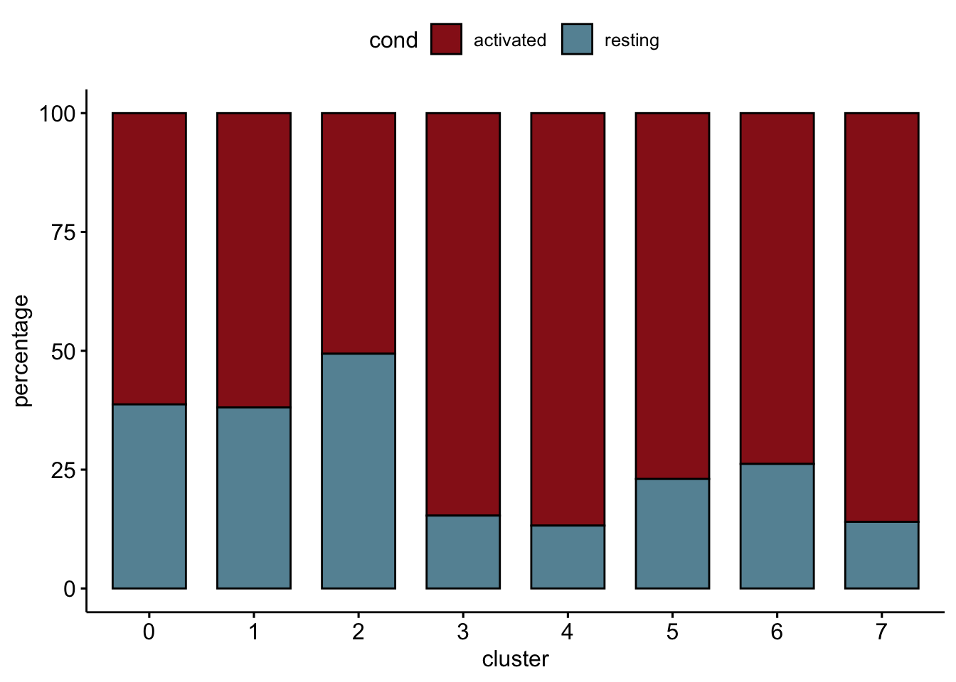
## relative abundance per cond
clustCond <- data.frame(table(seuratSub$cond2, seuratSub$intCluster))
colnames(clustCond) <- c("cond", "intCluster", "cnt")
condTot <- data.frame(table(seuratSub$cond2))
colnames(condTot) <- c("cond", "tot")
colPaldat <- data.frame(col=colPal) %>%
  rownames_to_column(var = "intCluster")
clustDat2 <- clustCond %>%  left_join(., condTot, by = "cond") %>%
  mutate(relAb = cnt/tot * 100) %>%
  left_join(., colPaldat, by = "intCluster")

knitr::kable(clustDat2)| cond | intCluster | cnt | tot | relAb | col |
|---|---|---|---|---|---|
| activated | 0 | 3464 | 18575 | 18.648721 | #800000FF |
| resting | 0 | 2189 | 7849 | 27.888903 | #800000FF |
| activated | 1 | 2327 | 18575 | 12.527591 | #767676FF |
| resting | 1 | 1431 | 7849 | 18.231622 | #767676FF |
| activated | 2 | 1990 | 18575 | 10.713324 | #FFA319FF |
| resting | 2 | 1941 | 7849 | 24.729265 | #FFA319FF |
| activated | 3 | 4021 | 18575 | 21.647375 | #8A9045FF |
| resting | 3 | 728 | 7849 | 9.275067 | #8A9045FF |
| activated | 4 | 2704 | 18575 | 14.557201 | #155F83FF |
| resting | 4 | 412 | 7849 | 5.249076 | #155F83FF |
| activated | 5 | 1664 | 18575 | 8.958277 | #C16622FF |
| resting | 5 | 498 | 7849 | 6.344757 | #C16622FF |
| activated | 6 | 1344 | 18575 | 7.235532 | #6692a3 |
| resting | 6 | 477 | 7849 | 6.077207 | #6692a3 |
| activated | 7 | 1061 | 18575 | 5.711978 | #3b7f60 |
| resting | 7 | 173 | 7849 | 2.204102 | #3b7f60 |
lapply(names(colCond2), function(co){
  clustDat2sel <- clustDat2 %>% filter(cond==co)
  pie(clustDat2sel$relAb,
      labels = clustDat2sel$intCluster,
      col = clustDat2sel$col,
      main = paste0(co, "- only same sorting"))
  symbols(0, 0, circles = 1, add=TRUE, bg="white")
})
[[1]]
NULL

[[2]]
NULLlapply(names(colCond2), function(co){
clustDat2sel <- clustDat2 %>% filter(cond==co)
pie(clustDat2sel$relAb,
labels = clustDat2sel$intCluster,
col = clustDat2sel$col,
main = paste0(co, "- only same sorting"))
})
[[1]]
NULL

[[2]]
NULL
relative cluster abundances per patient
clustCond <- data.frame(table(seurat$patient, seurat$intCluster))
colnames(clustCond) <- c("patient", "intCluster", "cnt")
clustTot <- data.frame(table(seurat$patient))
colnames(clustTot) <- c("patient", "tot")
patCond <- data.frame(seurat$patient, seurat$cond2) %>% unique()
colnames(patCond) <- c("patient", "cond")
clustDat <- clustCond %>%  left_join(., clustTot, by = "patient") %>%
  mutate(relAb = cnt/tot * 100) %>% left_join(., patCond, by = "patient")

ggbarplot(clustDat, x="patient", y="relAb",
          width = NULL,
          fill="intCluster",
          colour= "intCluster",
          palette = colPal,
          xlab = "patient",
          ylab = "percentage",
          legend = "right",
          legend.title = "") +
  rotate_x_text(angle = 90) +
  facet_grid(~cond, scales = "free", space = "free")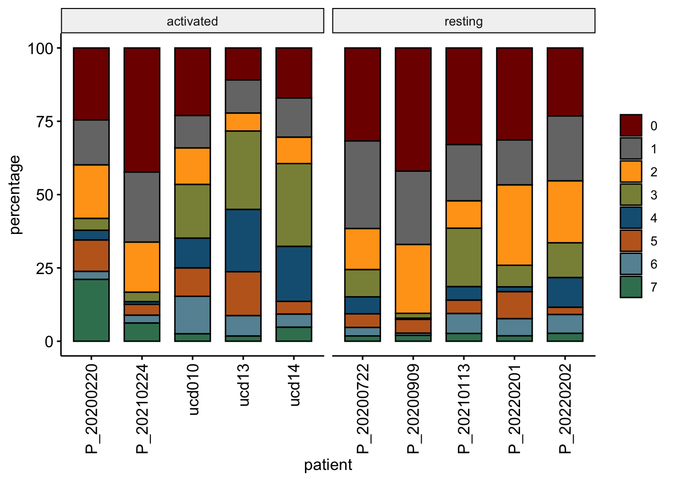
vis overall DE genes
marker genes
Idents(seurat) <- seurat$cond2
seurat_markers_all <- FindAllMarkers(object = seurat, assay ="RNA",
only.pos = TRUE, min.pct = 0.25,
logfc.threshold = 0.25,
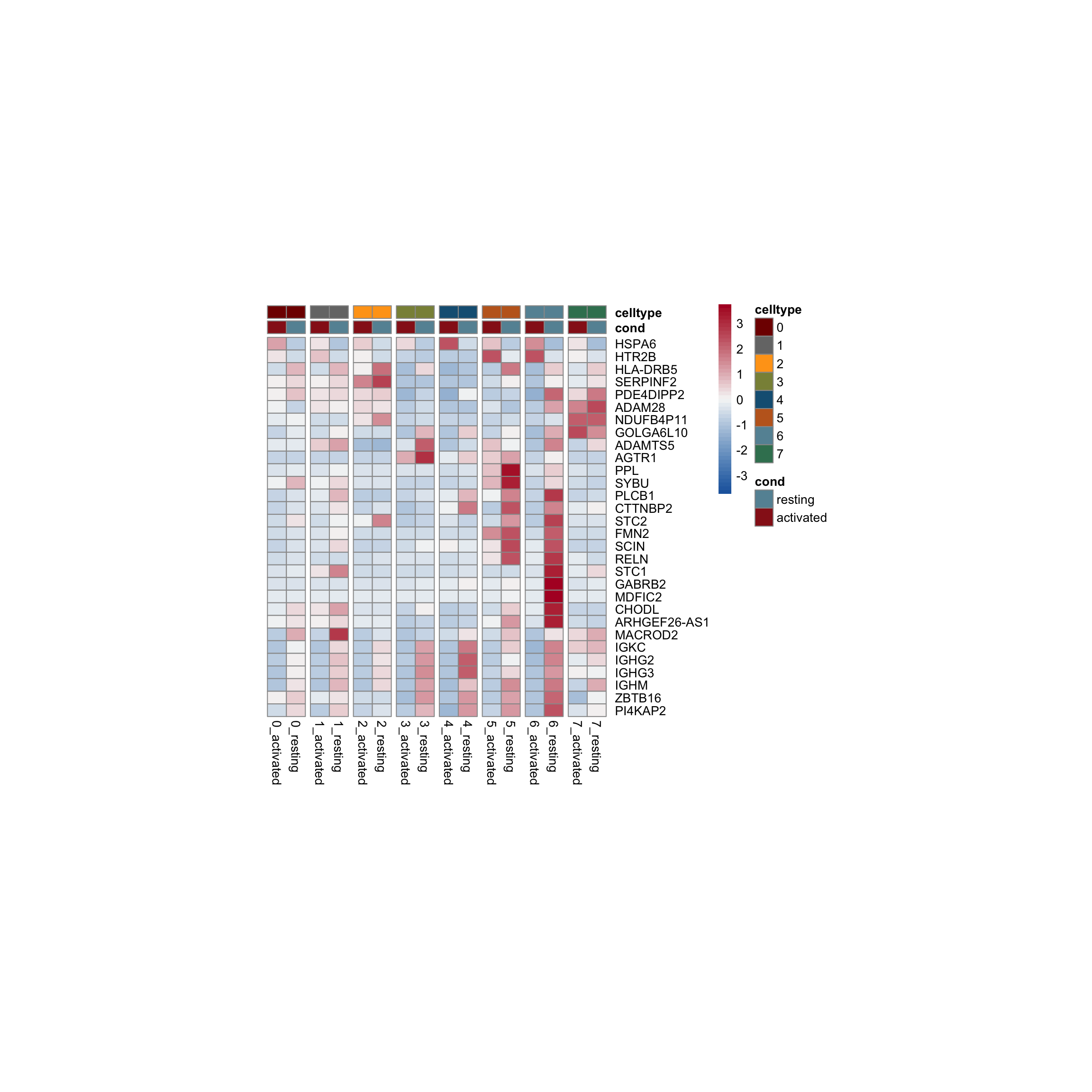
test.use = "wilcox")avg heatmap
cluster <- levels(seurat)
selGenesAll <- seurat_markers_all %>% group_by(cluster) %>%
  top_n(-15, p_val_adj) %>%
  top_n(15, avg_log2FC)
selGenesAll <- selGenesAll %>% mutate(geneIDval=gsub("^.*\\.", "", gene)) %>% filter(nchar(geneIDval)>1)

seurat$clust_plus_cond <- paste0(seurat$intCluster, "_", seurat$cond2)
Idents(seurat) <- seurat$clust_plus_cond
pOut <- avgHeatmap(seurat = seurat, selGenes = selGenesAll,
                  colVecIdent = colPal,
                  ordVec=levels(seurat),
                  gapVecR=NULL, gapVecC=NULL,cc=FALSE,
                  cr=T, condCol=T, colVecCond = colCond2)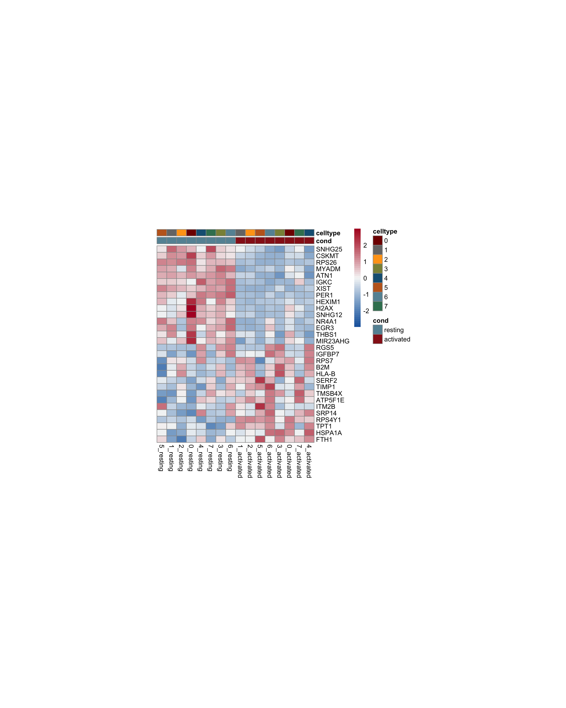
sc Heatmap
DefaultAssay(object = seurat) <- "RNA"
seurat <- ScaleData(seurat, features = rownames(seurat))

### plot DE genes top 25 avg logFC
DEGenesAll <- seurat_markers_all %>% group_by(cluster) %>%
  top_n(30, avg_log2FC)

selFeatures <- DEGenesAll %>% mutate(label=gsub("^.*\\.", "", gene))
DoHeatmap(seurat, features = selFeatures$gene, group.by = "cond2",
          group.colors = colCond2, slot = 'scale.data', label = F,
          disp.min = -0.5, disp.max = 1.5) +
  scale_fill_continuous(type = "viridis") +
  scale_y_discrete(breaks=selFeatures$gene, labels=selFeatures$label)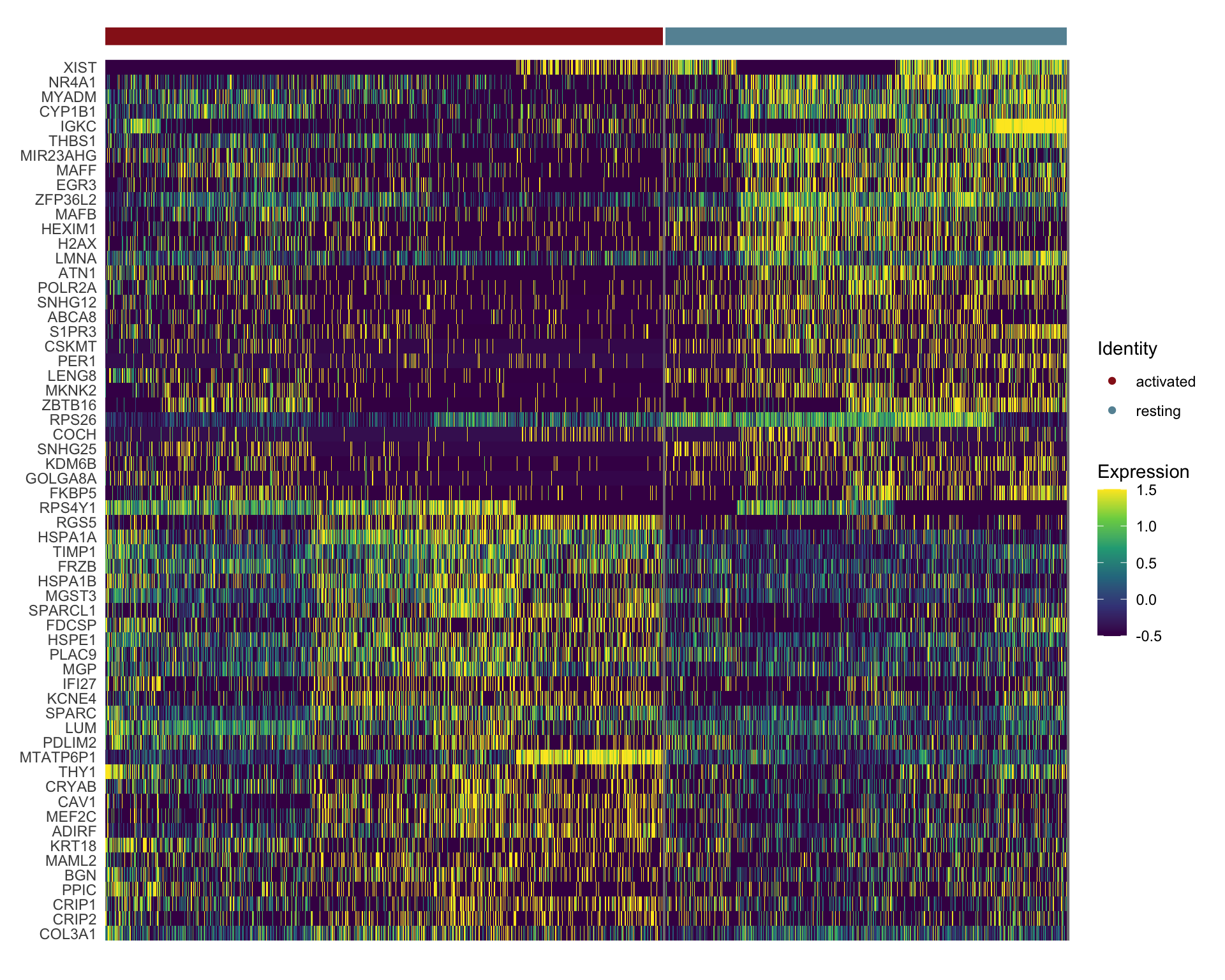
cw DE genes
Idents(seurat) <- seurat$cond2
grpVec <- unique(seurat$intCluster)
clustDE <- lapply(grpVec, function(grp){
grpSub <- unique(seurat$intCluster)[which(
unique(seurat$intCluster)==grp)]
seuratSub <- subset(seurat, intCluster == grpSub)
DEgenes <-FindAllMarkers(seuratSub, only.pos=T, logfc.threshold = 0.1,
min.pct = 0.01)
if(nrow(DEgenes)>1){
DEgenes <- DEgenes %>% filter(p_val_adj<0.01) %>%
mutate(group=paste0(grp, "_", cluster)) %>%
mutate(geneID=gsub(".*\\.", "", gene)) %>%
filter(nchar(geneID)>1)
}
})
names(clustDE) <- grpVec
clustDE_Dat <- data.frame(do.call("rbind", clustDE))
write.table(clustDE_Dat,
file=paste0(basedir, "/data/AllPatWithoutCM_FRConly_intOrig_cond2",
"_cwDEGenes.txt"),
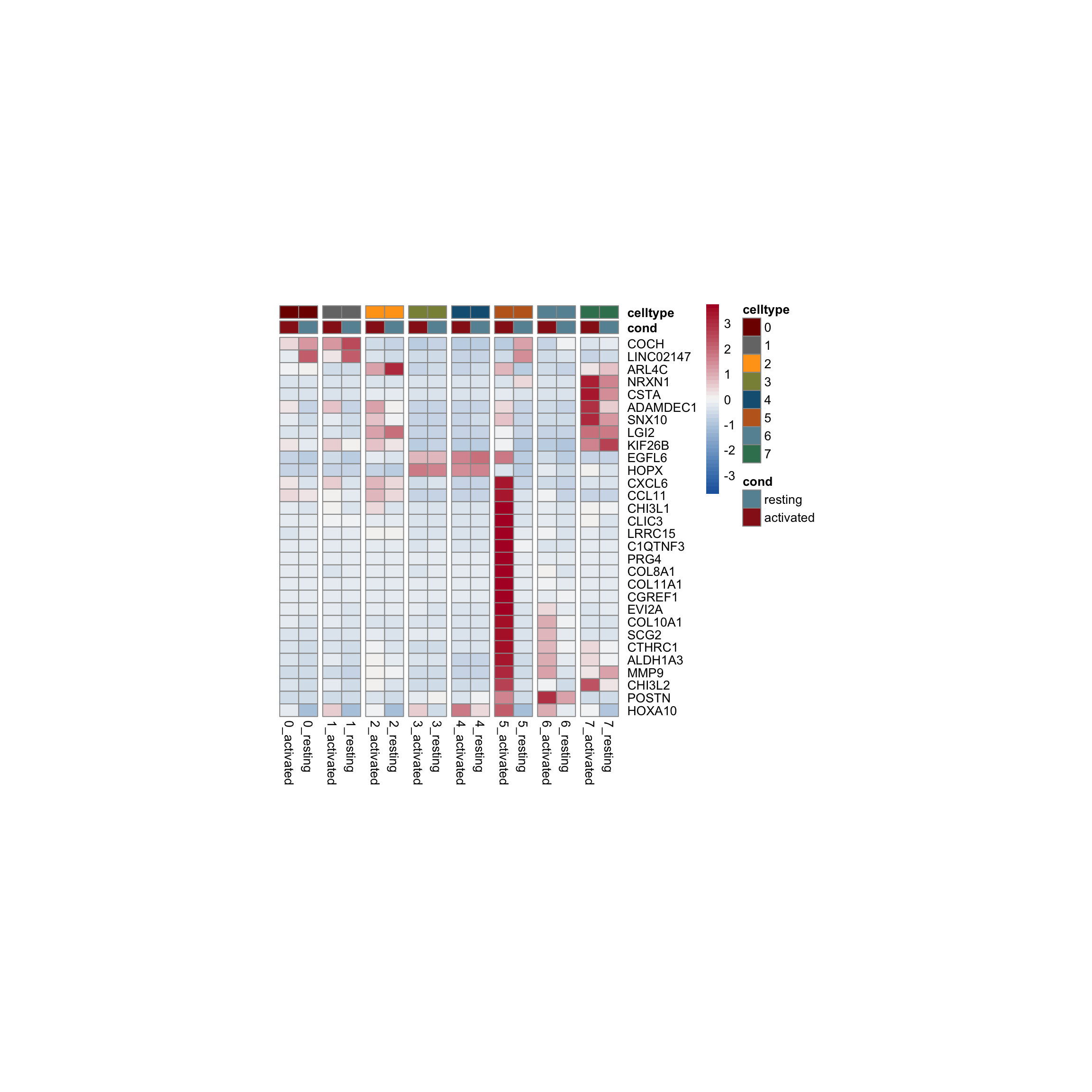
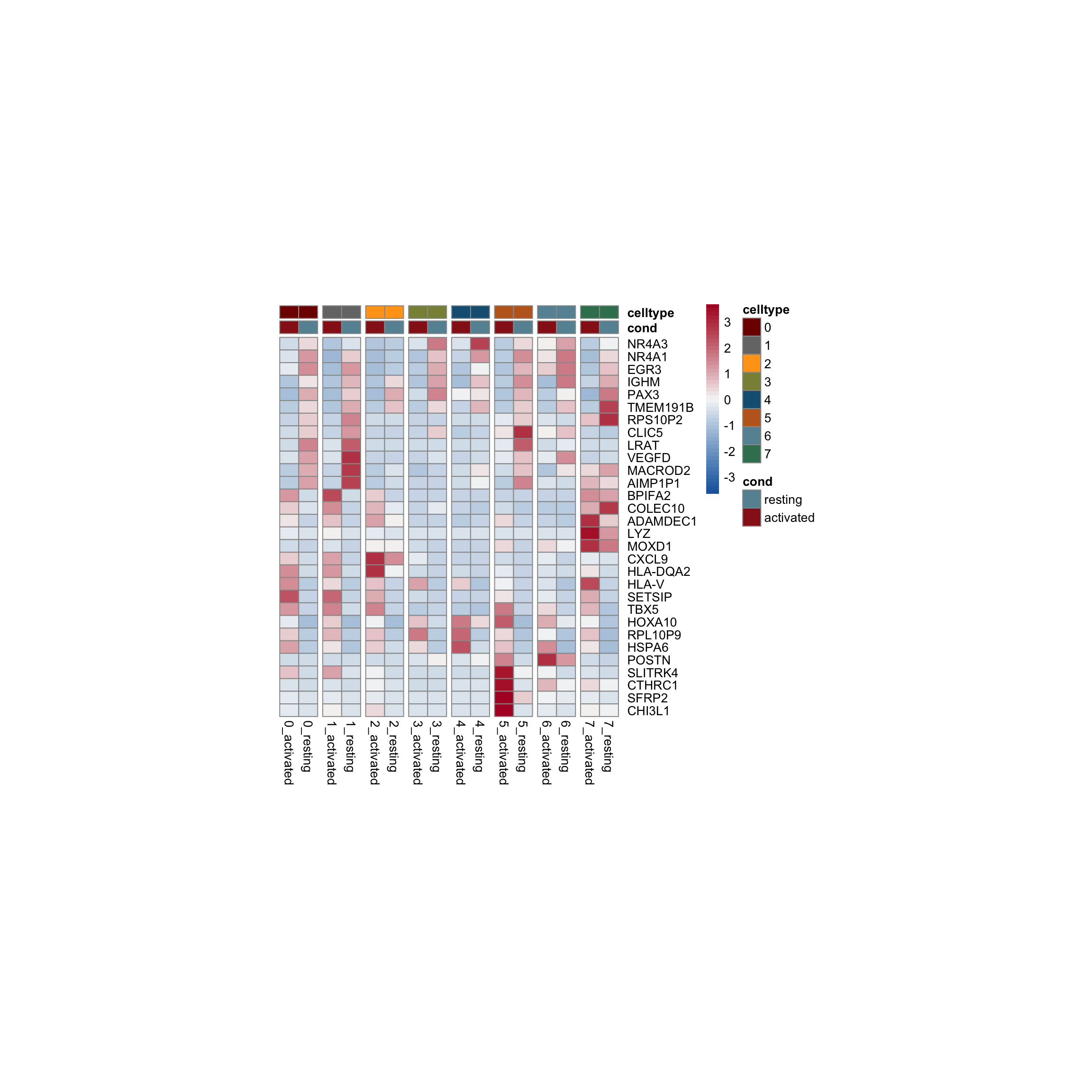
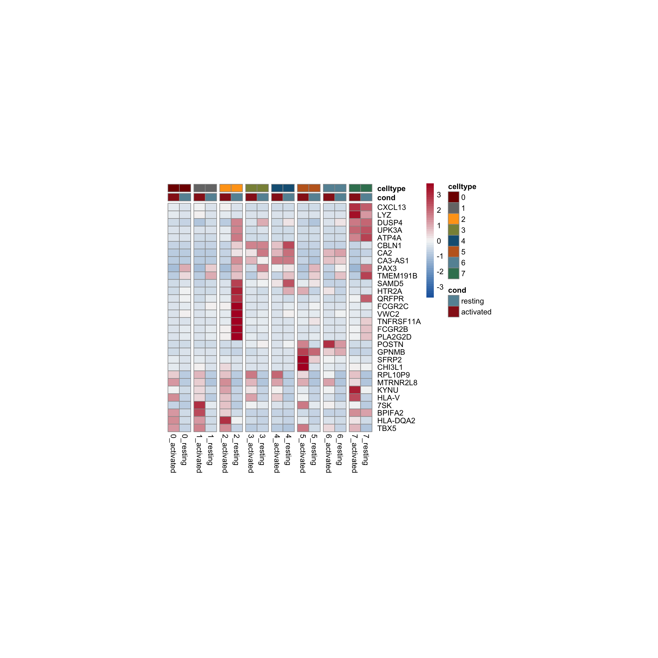
row.names = FALSE, col.names = TRUE, quote = FALSE, sep = "\t")avg Heatmap top cwDE genes
5
1
2
0
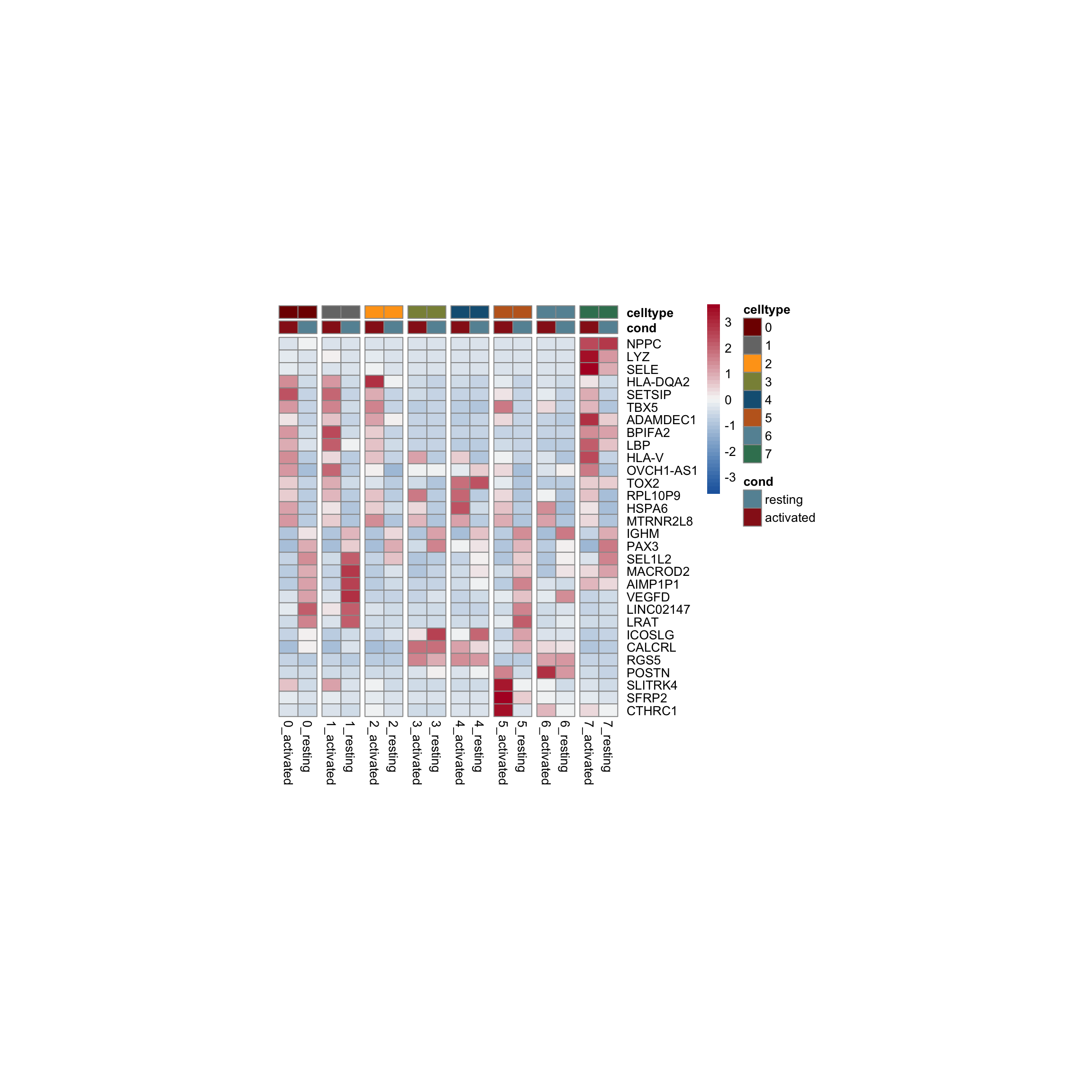
4
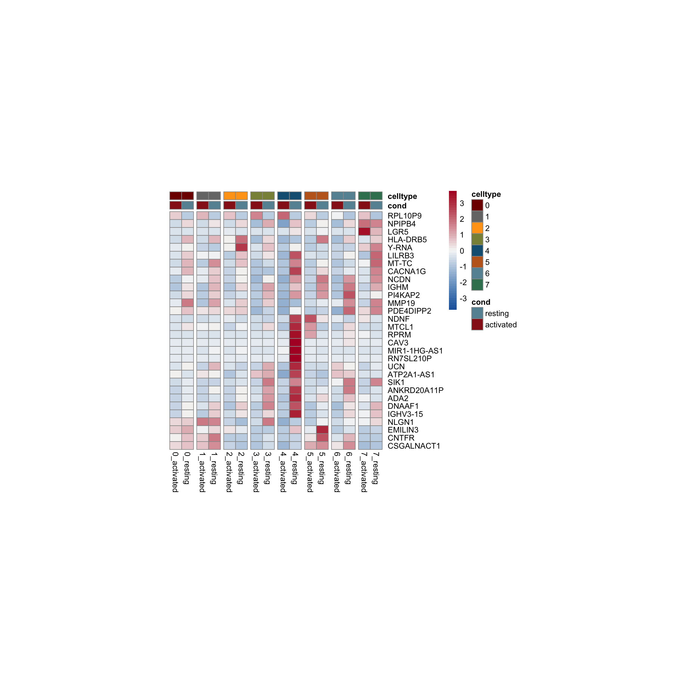
7
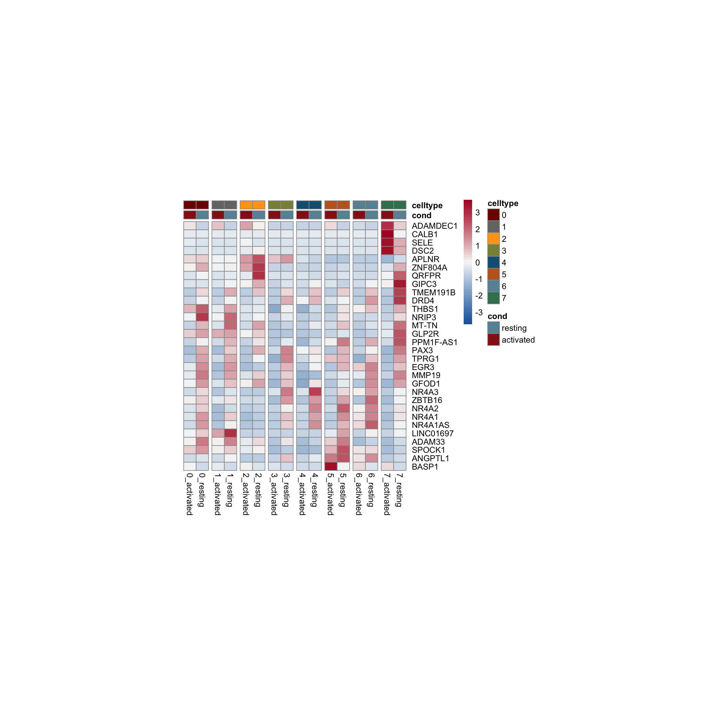
3
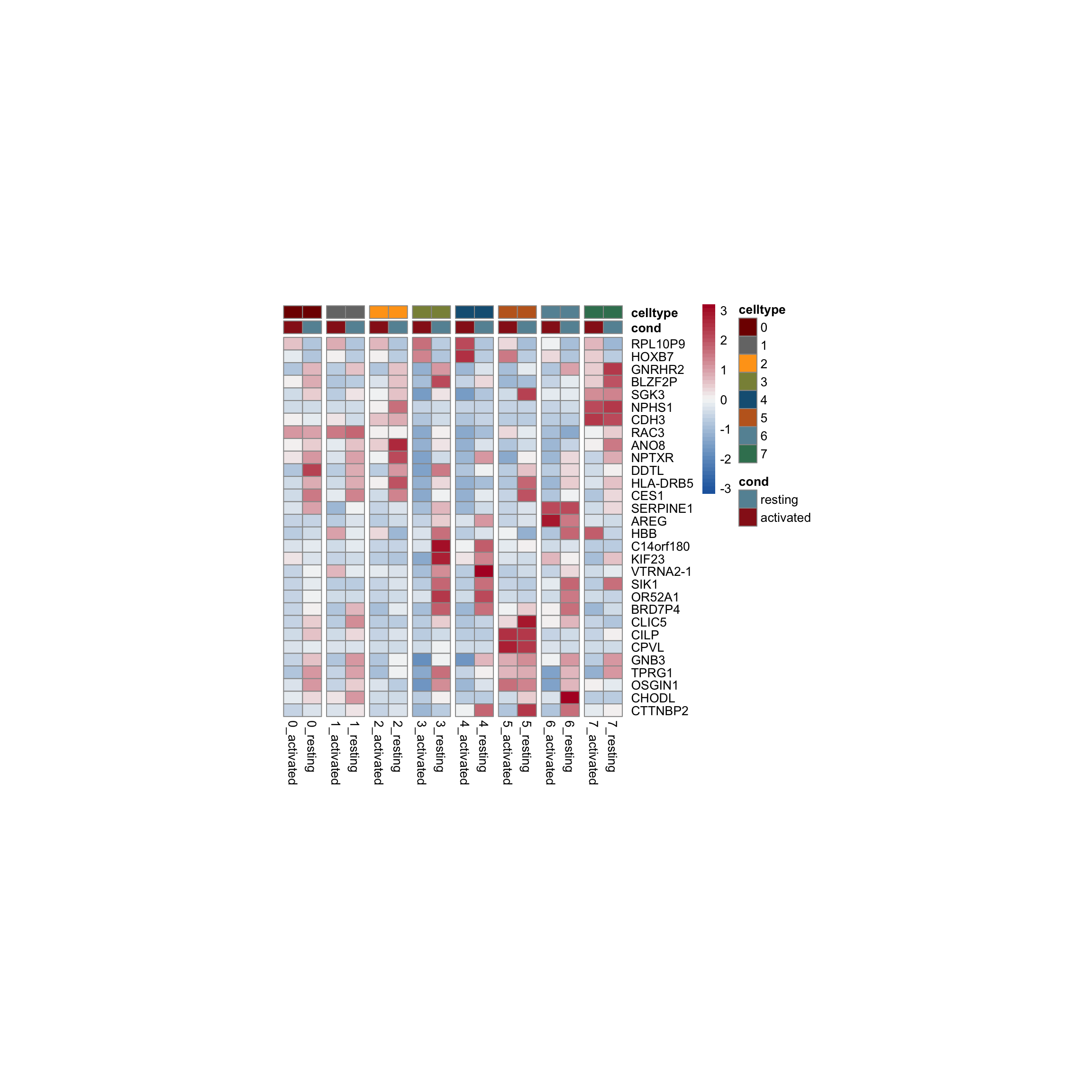
6
scatterplot cw DE genes cond 2
## scatterplot
## in red are all genes with an adjusted p_val < 0.01 and avg_logFC >0.25

################################################################################
### include only genes expressed in at least 10 % of cells in one condition ####
################################################################################
grpVec <- unique(seurat$integrated_snn_res.0.25)

lapply(grpVec, function(x){
  allID <- subset(seurat, integrated_snn_res.0.25 == x)
  Idents(allID) <-allID$cond2
  avg.allID <- AverageExpression(allID, group.by="cond2",
                                 show.progress = FALSE)
  avg.allID <- data.frame(log1p(avg.allID$RNA)) %>%
    rownames_to_column(var="gene")

  ## expression frequency
  GeneFreqSel <- as.data.frame(GetAssayData(allID, assay = "RNA",
                                            slot = "data")) %>%
    tibble::rownames_to_column(var="gene") %>% mutate(count=rowSums(.!=0)-1) %>%
    mutate(countFreq=count/ncol(allID)) %>%
    dplyr::select(gene,count, countFreq) %>%
    dplyr::filter(countFreq>=0.1)

  signGenes2 <- clustDE_Dat %>% mutate(grp=gsub("_.*", "", group)) %>%
    dplyr::filter(grp == x) %>%
    dplyr::filter(p_val_adj<0.01 & (avg_log2FC > 0.25))

  genes.to.label <- signGenes2 %>% group_by(.,cluster) %>%
    slice_max(avg_log2FC, n=15) %>% mutate(labelNam=geneID)

  avg.allID <- avg.allID %>% mutate(labelNam=gsub("^.*\\.", "", gene)) %>%
    mutate(colourGrp=ifelse(gene %in% genes.to.label$gene, "lab",
                            ifelse(gene%in%signGenes2$gene, "sig", "notSig"))) %>%
    dplyr::filter(gene%in%GeneFreqSel$gene)


  p_allID <- ggscatter(avg.allID, x="resting", y="activated",
                      color = "colourGrp",
                      palette = c("#660000", "#808080", "#FF3333"),
                      label="labelNam",
                      label.select = genes.to.label$labelNam,
                      repel = F,
                      label.rectangle=F,
                      xlab="resting",
                      ylab = "activated",
                      title=paste0("average expression - cluster ", x),
                      legend="none",
                      font.label=10,
                      alpha=0.9,
                      size=0.5)

  p_allID

})
[[1]]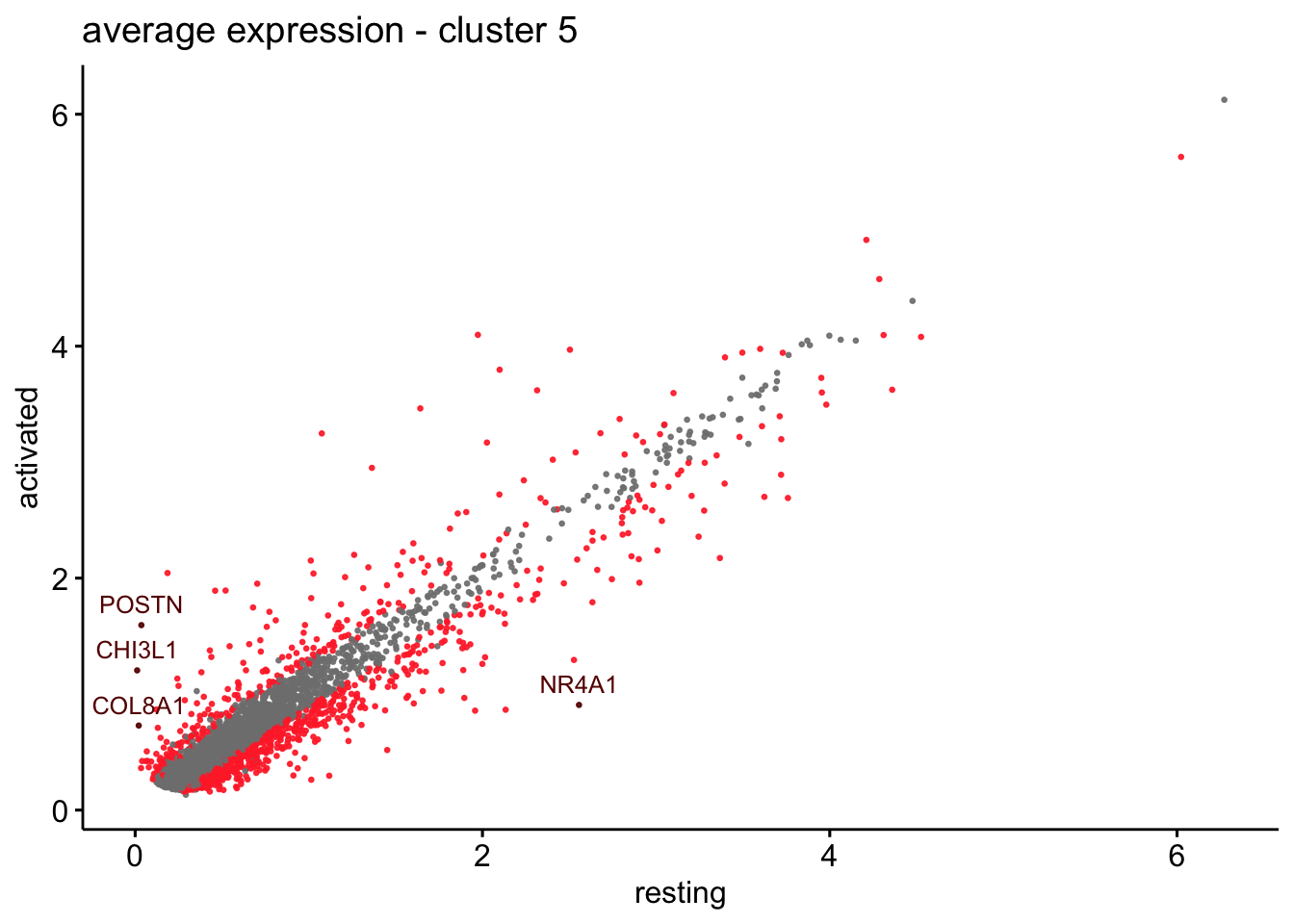
[[2]]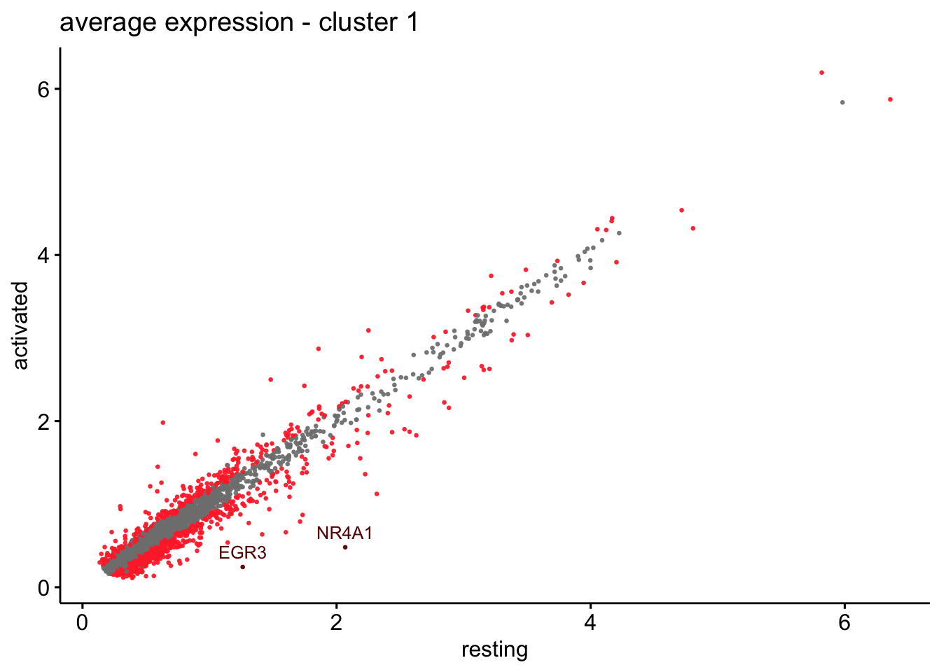
[[3]]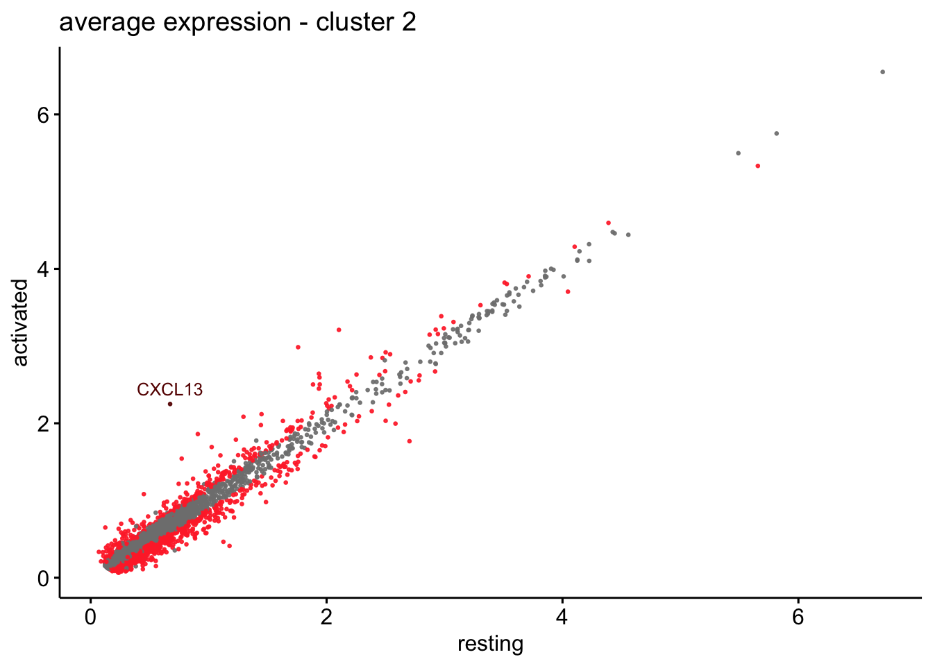
[[4]]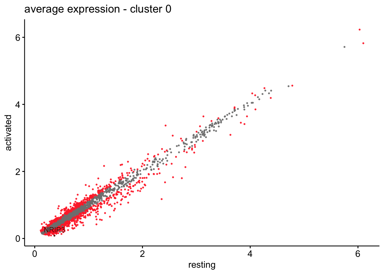
[[5]]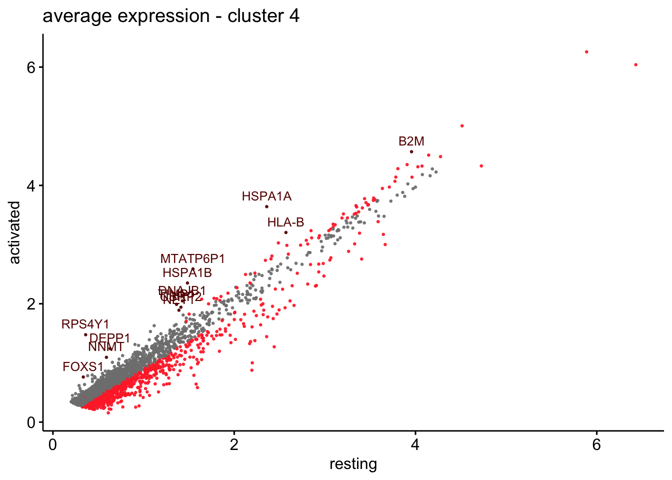
[[6]]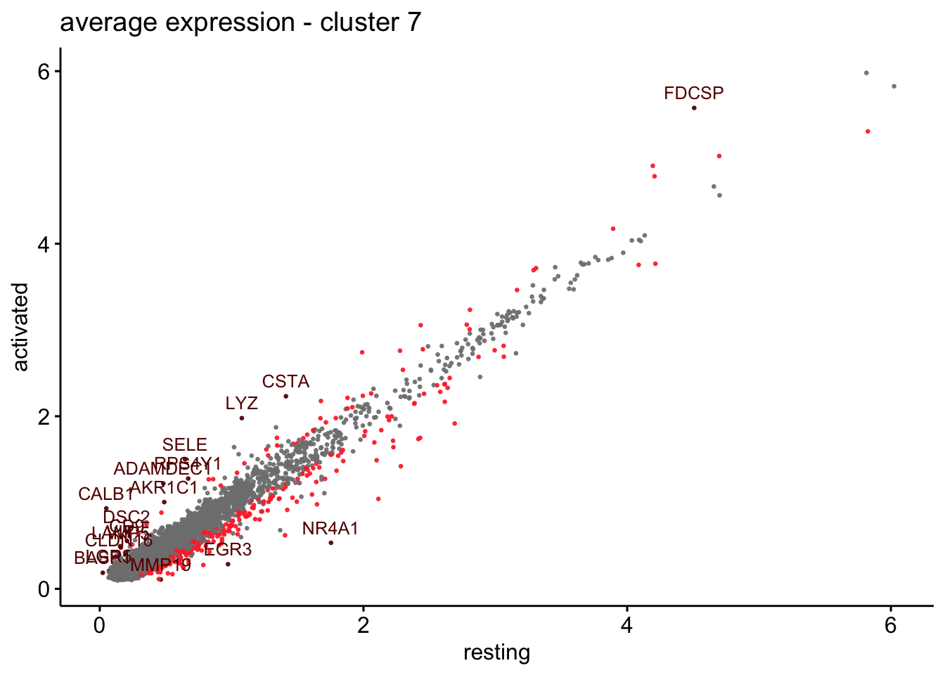
[[7]]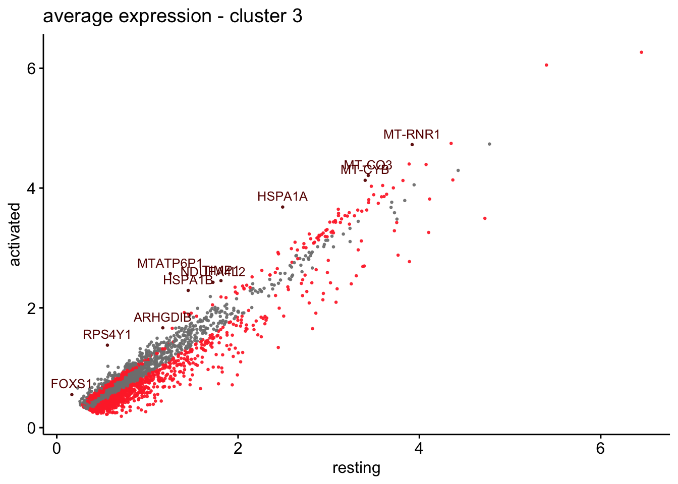
[[8]]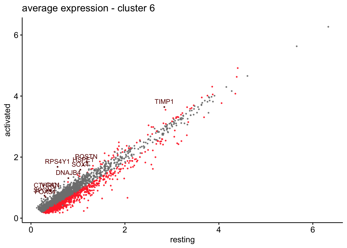
sc heatmap across all top cw DE genes
colPal2 <- rep(colPal, each=2)
names(colPal2) <- as.vector(t(outer(names(colPal), names(colCond2), paste,
                                    sep="_")))

### plot DE genes top 15 avg logFC
DEGenesAll <- clustDE_Dat %>% group_by(group) %>%
  top_n(15, avg_log2FC)

selFeatures <- DEGenesAll %>% mutate(label=gsub("^.*\\.", "", gene))
DoHeatmap(seurat, features = unique(selFeatures$gene),
          group.by = "clust_plus_cond",
          group.colors = colPal2, slot = 'scale.data', label = F,
          disp.min = -0.5, disp.max = 1.5) +
  scale_fill_continuous(type = "viridis") +
  scale_y_discrete(breaks=selFeatures$gene, labels=selFeatures$label)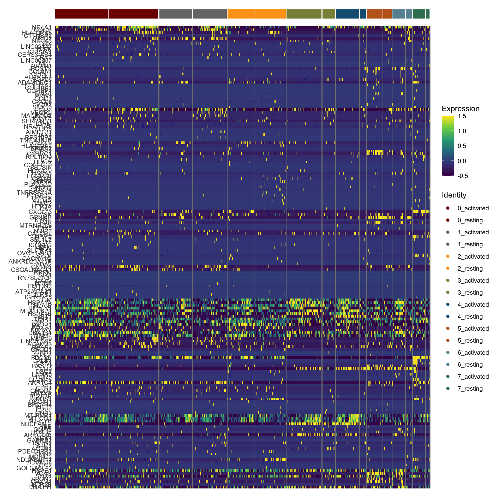
session info
sessionInfo()R version 4.3.0 (2023-04-21)
Platform: x86_64-apple-darwin20 (64-bit)
Running under: macOS Ventura 13.4.1
Matrix products: default
BLAS: /Library/Frameworks/R.framework/Versions/4.3-x86_64/Resources/lib/libRblas.0.dylib
LAPACK: /Library/Frameworks/R.framework/Versions/4.3-x86_64/Resources/lib/libRlapack.dylib; LAPACK version 3.11.0
locale:
[1] en_US.UTF-8/en_US.UTF-8/en_US.UTF-8/C/en_US.UTF-8/en_US.UTF-8
time zone: Europe/Berlin
tzcode source: internal
attached base packages:
[1] stats4 stats graphics grDevices utils datasets methods base
other attached packages:
[1] scater_1.28.0 scuttle_1.10.3 SingleCellExperiment_1.22.0
[4] SummarizedExperiment_1.30.2 Biobase_2.60.0 GenomicRanges_1.52.1
[7] GenomeInfoDb_1.36.4 IRanges_2.36.0 S4Vectors_0.40.1
[10] BiocGenerics_0.48.0 MatrixGenerics_1.12.3 matrixStats_1.2.0
[13] pheatmap_1.0.12 ggsci_3.0.1 here_1.0.1
[16] runSeurat3_0.1.0 ggpubr_0.6.0 lubridate_1.9.3
[19] forcats_1.0.0 stringr_1.5.1 readr_2.1.5
[22] tidyr_1.3.1 tibble_3.2.1 tidyverse_2.0.0
[25] Seurat_5.0.2 SeuratObject_5.0.1 sp_2.1-3
[28] purrr_1.0.2 cowplot_1.1.3 ggplot2_3.5.0
[31] reshape2_1.4.4 dplyr_1.1.4
loaded via a namespace (and not attached):
[1] RcppAnnoy_0.0.22 splines_4.3.0 later_1.3.2
[4] bitops_1.0-7 polyclip_1.10-6 fastDummies_1.7.3
[7] lifecycle_1.0.4 rstatix_0.7.2 rprojroot_2.0.4
[10] globals_0.16.2 lattice_0.22-5 MASS_7.3-60.0.1
[13] backports_1.4.1 magrittr_2.0.3 limma_3.56.2
[16] plotly_4.10.4 rmarkdown_2.26 yaml_2.3.8
[19] httpuv_1.6.14 sctransform_0.4.1 spam_2.10-0
[22] spatstat.sparse_3.0-3 reticulate_1.35.0 pbapply_1.7-2
[25] RColorBrewer_1.1-3 abind_1.4-5 zlibbioc_1.46.0
[28] Rtsne_0.17 presto_1.0.0 RCurl_1.98-1.14
[31] GenomeInfoDbData_1.2.10 ggrepel_0.9.5 irlba_2.3.5.1
[34] listenv_0.9.1 spatstat.utils_3.0-4 goftest_1.2-3
[37] RSpectra_0.16-1 spatstat.random_3.2-3 fitdistrplus_1.1-11
[40] parallelly_1.37.1 DelayedMatrixStats_1.22.6 leiden_0.4.3.1
[43] codetools_0.2-19 DelayedArray_0.26.7 tidyselect_1.2.0
[46] farver_2.1.1 viridis_0.6.5 ScaledMatrix_1.8.1
[49] spatstat.explore_3.2-6 jsonlite_1.8.8 BiocNeighbors_1.18.0
[52] ellipsis_0.3.2 progressr_0.14.0 ggridges_0.5.6
[55] survival_3.5-8 tools_4.3.0 ica_1.0-3
[58] Rcpp_1.0.12 glue_1.7.0 gridExtra_2.3
[61] xfun_0.42 withr_3.0.0 fastmap_1.1.1
[64] fansi_1.0.6 rsvd_1.0.5 digest_0.6.34
[67] timechange_0.3.0 R6_2.5.1 mime_0.12
[70] colorspace_2.1-0 scattermore_1.2 tensor_1.5
[73] spatstat.data_3.0-4 utf8_1.2.4 generics_0.1.3
[76] data.table_1.15.2 httr_1.4.7 htmlwidgets_1.6.4
[79] S4Arrays_1.0.6 uwot_0.1.16 pkgconfig_2.0.3
[82] gtable_0.3.4 lmtest_0.9-40 XVector_0.40.0
[85] htmltools_0.5.7 carData_3.0-5 dotCall64_1.1-1
[88] scales_1.3.0 png_0.1-8 knitr_1.45
[91] rstudioapi_0.15.0 tzdb_0.4.0 nlme_3.1-164
[94] zoo_1.8-12 KernSmooth_2.23-22 vipor_0.4.7
[97] parallel_4.3.0 miniUI_0.1.1.1 pillar_1.9.0
[100] grid_4.3.0 vctrs_0.6.5 RANN_2.6.1
[103] promises_1.2.1 BiocSingular_1.16.0 car_3.1-2
[106] beachmat_2.16.0 xtable_1.8-4 cluster_2.1.6
[109] beeswarm_0.4.0 evaluate_0.23 cli_3.6.2
[112] compiler_4.3.0 rlang_1.1.3 crayon_1.5.2
[115] future.apply_1.11.1 ggsignif_0.6.4 labeling_0.4.3
[118] ggbeeswarm_0.7.2 plyr_1.8.9 stringi_1.8.3
[121] BiocParallel_1.34.2 viridisLite_0.4.2 deldir_2.0-4
[124] munsell_0.5.0 lazyeval_0.2.2 spatstat.geom_3.2-9
[127] Matrix_1.6-5 RcppHNSW_0.6.0 hms_1.1.3
[130] patchwork_1.2.0 sparseMatrixStats_1.12.2 future_1.33.1
[133] shiny_1.8.0 ROCR_1.0-11 igraph_2.0.2
[136] broom_1.0.5 date()[1] "Wed Mar 13 19:07:39 2024"